
Background
When selecting a dataset for a case study in biotech, it was important to find something unique to the domain. Ideally, we utilize a task with many and sparse features, difficult to discern signal-to-noise ratio, and a small number of examples. These are key characteristics of this dataset of cancer inhibitor protein interactions.
How useful is the Ensemble ‘Dark Matter’ algorithm and can it be used on data of this format? What kinds of downstream model improvements or detriments are observed while applying Ensemble to the training pipeline? What ratio of bias/variance is observed in the downstream models before and after using Ensemble? Keep these questions in mind as we explore the results.
Dataset

Small molecules play an non-trivial role in cancer chemotherapy. Here [the dataset owner will] focus on inhibitors of 8 protein kinases(name: abbr):
- Cyclin-dependent kinase 2: cdk2
- Epidermal growth factor receptor erbB1: egfr_erbB1
- Glycogen synthase kinase-3 beta: gsk3b
- Hepatocyte growth factor receptor: hgfr
- MAP kinase p38 alpha: map_k_p38a
- Tyrosine-protein kinase LCK: tpk_lck
- Tyrosine-protein kinase SRC: tpk_src
- Vascular endothelial growth factor receptor 2: vegfr2
For each protein kinase, several thousand inhibitors are collected from chembl database, in which molecules with IC50 lower than 10 uM are usually considered as inhibitors, otherwise non-inhibitors.
Based on those labeled molecules, build your model, and try to make the right prediction.
Additionally, more than 70,000 small molecules are generated from pubchem database. And you can screen these molecules to find out potential inhibitors. P.S. the majority of these molecules are non-inhibitors.
Dataset Info
- 1890 examples
- 6117 sparse features
- After split
- training set shape:
(1790, 6117) - test set shape:
(100, 6117)
- training set shape:
- Total target counts:
All:
1      1271
0      619
Train:
1 1199
0 591
Test:
1 72
0 28
The imbalance in the target values is around 4:1, not significant enough to require dataset balancing techniques like over/under sampling.
- Sparcity:
(X_train.sum(axis=0) / X_train.shape[0]).mean()
>> 0.25362096474428353
A quick check shows us that on average, each feature in this dataset has
- 25% (450 / 6000) 1s
- 75% (5545 / 6000) 0s
- Nulls:
pd.DataFrame(X_train).isnull().sum().sum()
>> 0
Metrics comparison
- Compares baseline metrics (no Ensemble AI used) to Ensemble metrics (using Ensemble AI to preprocess input features)

- Original feature count: 6117
- Ensemble embedding size: 50
- Ensemble training iteration count: 10,000 epochs
This configuration, when using Ensemble, functions as both feature enhancement as well as dimensionality reduction for very large, sparse vectors.
Ex:
Baseline modeling pipeline
→ <6117 features> → model → prediction
Ensemble modeling pipeline
→ <6117 features> → Ensemble → <50 features> → model → predictionMetric Slope Plots
Metric Slope Plots
The following plots show the performance change before and after using Ensemble for a variety of metrics:
→ Accuracy, Precision, Recall, AUC, F1, and Specificity.
The downstream models tested include a collection of both linear and non-linear classification algorithms:
→ Logistic Regression, Random Forest, XGBoost, CatBoost, Support Vector Machine Classification, and Multi-Layer Perceptron.
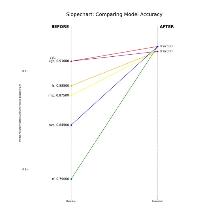
Models typically improve, with many achieving similar accuracy. In future work, we will monitor metrics as we increase the holdout set size.
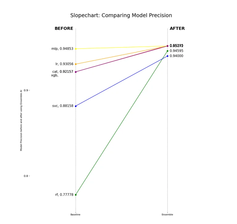
Precision remains steady across different models. This means that with Ensemble, almost any downstream model can achieve good precision with this holdout set size.
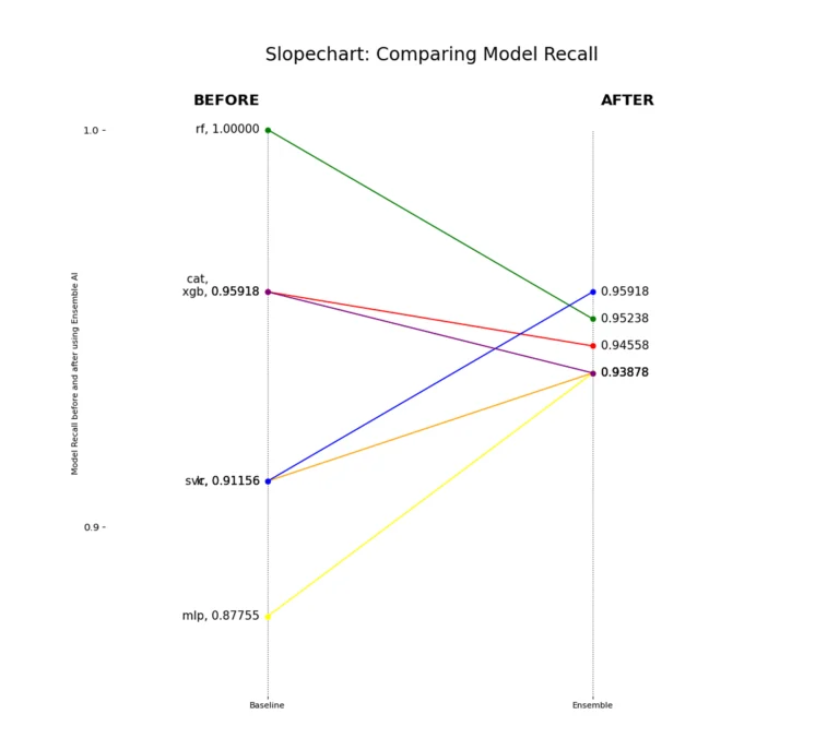
Recall stays consistent across all models. This means that detecting false positives is congruent no matter which downstream model is used when training with enhanced features from the Ensemble algorithm.
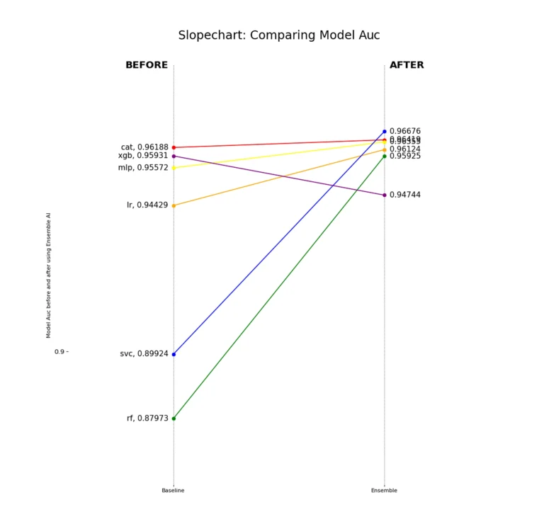
The ROC AUC shrinks for some boosting algorithms, but grows for other linear and non-linear algorithms used as the downstream model. In future work, testing other classification thresholds could reveal better ROC AUC scores for each downstream model.
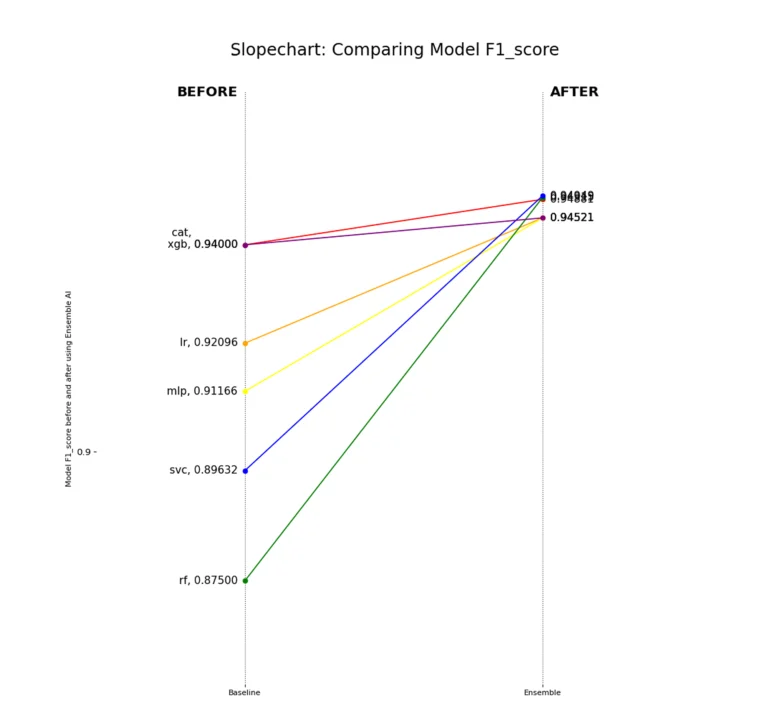
The F1 score stays steady across models, showing that using Ensemble improves both precision and recall for any downstream model.
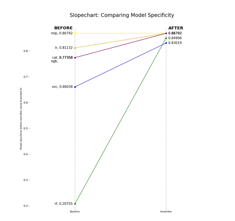
Looking at the True Negative Rate (Specificity) shows that some models predict the majority class (1s) too often. Sometimes, they act like a single-value predictor (like Random Forest). Using Ensemble emphasizes variance in the data, even with few data points and dataset imbalance.
Conclusion
This case study shows the benefit of using the Ensemble ‘Dark Matter’Dark Matter algorithm to generate embeddings in a domain with sparse and limited data. The algorithm highlights points of variance that are otherwise lost on common and uncommon brands of machine learning algorithms.
Random Forest struggled to predict effectively, and would likely be discarded after this baseline test in another experiment. However, when given the opportunity to understand the dataset’s variance at a deeper level, Random Forest and other linear and non-linear algorithms are all able to converge on a similar high performance model.